Introduction

The capacity to accurately assess the system’s performance is a crucial first step in developing an ML system. Although the selection of an evaluation measure depends on the context, accuracy, precision, and recall are the preferred metrics for the majority of ML models, such as binary or multi-class classifiers (also the subject of this article). All we need is “large enough” labeled data and apply the formulae. Larger the test data, accurate the performance metrics. However, there are several issues with this. First, we are unsure of the size at which we can confidently assess the metrics; and second, there may be circumstances in which we are unable to have huge amounts of labeled test data (e.g. labeling cost is high). This is where confidence intervals (CI) come in. Consider the following two cases:

Case 1: Model A has a precision of 0.78 and Model B has a precision of 0.81.
Case 2: Model A precision lies in the interval (0.76, 0.80) with 95% probability. Model B precision lies in the interval (0.77, 0.83) with 95% probability.

In case 1, Model B is certainly superior than Model A, but when we look at the spread of precision for model B in case 2, Model B might be worse than Model A.

In this post, I will discuss two approaches to find the confidence intervals, namely the non-parametric bootstrap method, and the parametric modeling method. This will be followed by a derivation of confidence intervals for precision and recall with the parametric modeling approach.

Non parametric versus parametric approach

There are mainly two approaches to compute the CIs for a given estimate:

The first approach is not assuming any underlying process that generates the data. An example is the bootstrapping method where a sample of data is used to produce many re-samplings (with replacement). Estimates are computed using those re-samples.
The second approach is modeling the underlying data generating process, a.k.a parametric approach. Here, we find the parameters of an assumed distribution that models the estimate of interest.

When it comes to computing CIs using a non-parametric approach such as bootstrapping, there are two downsides:

When the sample is small, they perform poorly. This is going to be the case when the labeling process is expensive.
Makes no assumption of the underlying distribution even if useful information is available. This makes this approach unreliable in producing good CIs.

Although there are some disadvantages, it does have some advantages, mainly when the metric is arbitrary and there are no suitable modeling approaches. Here is a nice working article/library that use bootstrap method to compute the CIs for accuracy, precision and recall.

In the following sections, our discussion will primarily follow the parametric approach. We leave out the the CI computation for accuracy metrics because there are great resources that details it, for example here. We will see how inversion test (discussed here is used to derive the CIs of precision.

CIs for precision — The parametric approach

We define precision as:

\[\begin{equation} Precision = \frac{True Positive}{(True Positive + False Positive)} \end{equation}\]

Let’s denote the number of items labelled positive by the model as \(x_{precision}\) and total number of items labelled positive by the model as \(n_{precision}\). Also, let’s denote \(p_{precisiion}\) as the model of precision. Then,

\[\begin{equation} \hat{p}_{precision} = \frac{x_{precision}}{n_{precision}} \end{equation}\]

\(p_{precision}\) The underlying distribution that models the precision naturally follows a Binomial distribution.

\[\begin{equation} p_{precision} \sim p^{x_{precision}}*(1-p)^{n_{precision}-x_{precision}} \end{equation}\]

where \(p\) is the parameter of the precision model.

Binomial likelihood ratio test and the test inversion

A likelihood test statistics measures the distance between mostly likely parameter (MLE) and the observed parameter given an underlying distribution. To depict it graphically,

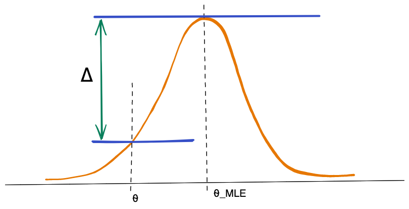
Cosidering that our null hypothesis is \(H_{0}: p = p_{0}\), then the larger the distance \(\triangle\), the higher the chance that the null hypothesis is rejected. In other words we keep all such p not such that we cannot reject the null hypothesis under the test statistics.

The likelihood test statistics is given by:

\[\begin{equation} LR(p_{0}) = 2*(l(\hat{p}_{precision}) - l(p_{0}))) \end{equation}\]

where \(l\) is the likelihood function. For a binomial distribution, the likelihood function is given by:

\[\begin{equation} l(p) = x_{precision} * log(p) + (n_{precision}-x_{precision}) * log(1-p) \end{equation}\]

An interesting thing about likelihood test is that it asymptotes to Chi-squared distribution with 1 degree of freedom (denoted by \(\chi^{2}_{1}\)). How? Checkout the derivation here.

Using the binomial likelihood function, the binomial likelihood ratio test statistics becomes:

\[\begin{equation} LR(p_{0}) = 2*(l(\hat{p}_{precision}) - l(p_{0}))) \\ = 2 (x_{precision} * log(\hat{p}_{precision}) + (n_{precision}-x_{precision}) * log(1-\hat{p}_{precision}) \\ - x_{precision} * log(p_{0}) + (n_{precision}-x_{precision}) * log(1-p_{0})) \\ = 2 \left( x_{precision} log\left(\frac{\hat{p}_{precision}}{p_{0}} \right) + (n_{precision} - x_{precision}) log\left( \frac{1-\hat{p}_{precision}}{1-p_{0}}\right)\right) \end{equation}\]

Since the test statistics is \(\chi^{2}_{1}\), we fail to reject the null hypothesis \(H_{0}\) for all such values of \(p_{0}\) that satisfies

\[\begin{equation} p_{0} \in (min_{p_{0}} s.t. LR(p_{0} \leq \chi^{2}_{1}), max_{p_{0}} s.t. LR(p_{0} \leq \chi^{2}_{1})) \end{equation}\]

Hence, the test inversion gives us the the confidence interval for precision as shown below:

\[\begin{equation} CI_{precision} = (min_{p_{0}} s.t. LR(p_{0} \leq \chi^{2}_{1}, max_{p_{0}} s.t. LR(p_{0} \leq \chi^{2}_{1})) \end{equation}\]

whith a certain confidence level \(\alpha\) that sets the the value of \(\chi^{2}_{1}\).

Let’s find the CI for Recall!

CIs for Recall — Monte Carlo simulation

Recall is define as:

\[\begin{equation} Recall = \frac{True Positive}{(True Positive + False Negative)} \end{equation}\]

The numerator and denominator are not independent. Moreover, the denominator require us to know the labeled data for full population. There is not way we can model this with any distribution.

Ouch!

Does that mean there is not way to find CIs for recall? No, we can! The technique here follows two steps:

Use independent parametric model(s) to model the recall.
Use monte carlo simulation to generate recall values and take the alpha percentile in order to create the confidence interval for recall.

Modeling Recall

It turns out that the recall can be modelled if we have a modelled the precision and negative predictive value.

\[\begin{equation} Negative predictive value = \frac{True Negative}{(True Negative + False Negative)} \\ = \frac{x_{npv}}{n_{nvp}} \end{equation}\]

where \(x_{nvp}\) is the total number of correctly negatively labelled items, and \(n_{nvp}\) is the total number of negative items that are labelled by the classifier.

Just like we found the model for precision, the model for negative predictive value also follows the binomial distribution. Now the main idea is to use precision and negative predictive value models to model the recall.

Recall can be re-written using the formulae of precision and NVP as follow (where \(N_{p}\) is total positiviely labelled items, and \(N\) is the total labelled items):

\[\begin{equation} Recall = \frac{Precision * N_{p}}{Precision * N_{p} + (1-NVP)*(N - N_{p})} \\ = \frac{\frac{True Positive * (True Positive + False Positive)}{(True Positive + False Positive)}}{\frac{True Positive * (True Positive + False Positive)}{(True Positive + False Positive)} + \frac{False Negative * (True Negative + False Negative)}{(True Negaive + False Negative)}}\\ = \frac{True Positive}{True Positive + False Negative} \end{equation}\]

Since the model for both precision and NVP are independent of each other, we use monte carlo simulation to generate \(N_{iter}\) samples of recall. Let’s assume that using the simulation, we have generate following sample and they are ordered in the increasing order \(R_{1}\), \(R_{2}\), \(R_{3}\), …, \(R_{N_{iter}}\), then the confidence interval for the recall is the \(\alpha\) and \(1-\alpha\) percentiles of the generated data.

Concluding thoughts

We presented the idea of computing confidence intervals for important ML evaluation metrics so that we can get a better picture of model performance. To do that, we looked into the the detail of how the CIs of accuracy, precision and recall is calculated. Code snippet to compute the CIs based on parametric approach will be update soon!

Notes

Please report errata and/or leave any comments/suggestion here.

Disclaimer: Information presented here does not represent views of my current or past employers. Opinions are my own.